


What exactly are algorithms? It is a series of actions taken to complete a task. For instance, if you were given a list of numbers and asked to provide the largest one, you would be able to answer that at first sight because there aren't many numbers, but the question is how you did it. Your eyes first gathered the information and transmitted it to your brain. The biggest number was then examined and stored by your brain. Now let's convert this to a language that the machine can comprehend. In this instance, I'm going to utilize Python.
# Where nums is an array (or collection) of numbers
def maximum(nums : list[int]) -> int:
    '''
        This function returns the greatest integer
        from an array of numbers.
    '''
    max  = 0 # variable to store the largest value
    # The array is first looped through (or scanned).
    for x in nums:
    # Next, we determine if each of the discovered numbers
    # is less than or equal to max.
        if max <= x:
            # If true then that number is our new max
            max = x
    # Return the largest number found (max at the end of the loop)
    return max
I decided to choose Python since I thought it was user-friendly and simple to comprehend.
Let's move on. Here comes the "tough" phase. The used algorithm unquestionably has a O(n) complexity. Ayy yo!, Let's briefly touch on this as it seems like I'm in a hurry. After all, O(n) is pronounced Big O of n. This notation, known as "Big O," is used to determine an algorithm's "asymptotic upper bound."
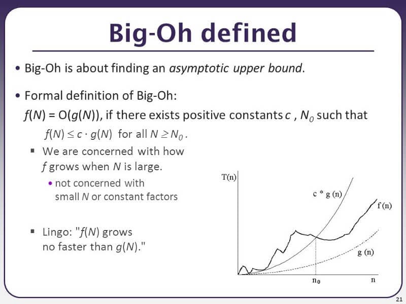
CSE 373 Slides from University of Washington
This formal representation is for a mathematical proof. This means that we are taking the performance of our algorithm to its bounding limits (or the limits of computer programming). Additionally, this demonstrates the algorithms' space-time complexity. The Space-Time Complexity reveals how much memory and time are required for an algorithm to execute a task. However, the "n" in this case indicates that even if our result might be at the beginning of the list, our algorithm will still need to deal with every element in the list. As a result, time and space are consumed and utilized proportionally to 'n' (the larger the 'n', the more memory and time consumed). This is not always the case; for example, a linear search algorithm has an O(n) complexity but stops when it finds the element we're looking for. The algorithm will have to search through the array until it reaches the end in the worst scenario, where the last value (in the array) is what we are seeking or the value provided is not present. Let's start by creating a Python linear search function before moving on to additional Big O-notable complexities.
# Where nums is a array (or collection) of numbers
# and target is a number (to be found)
def linearsearch(nums: list[int], target: int) -> int:
    '''
        This function takes an array of numbers ,
        the number to be found, and
        returns the index (position) of the target
        if found else
        returns -1
    '''
    # Firstly, we check for each value and it's index in the list
    for index, value in enumerate(nums):
        # Then we check if any of the values in the array is
        # equal to the target
        if value == target:
            # If that is true
            # return the index of the value
            return index
    # If not return -1
    return -1
NOTE: enumerate() is a Python built-in class that accepts an iterable (lists, tuples, dictionaries, and sets) as an argument and produces an iterable enumerate object that provides pairs comprising a count (from start, which defaults to zero) and a value returned by the iterable argument.
Moving on, because this is a brief article, I will only address the most common O(n) complexities. O(1) complexity is the simplest, requiring only one step to achieve the task at hand. The fact that it possesses "constant time" is also noteworthy. An example is using modulus (%) to check if a number is odd or even. Another complexity is O (log n), which is more complex than O(1) but less complex than O(n). The binary search algorithm is an illustration of this method, which includes splitting an array and comparing its center value to the target. The index of the value is then returned if the value is the target. If the target is smaller than the value, the first half of the array is taken. Additionally, the second half is taken if the target is higher than the value. The procedure is then carried out again, utilizing the selected half, until the desired outcome is attained. This is demonstrated in the code below.
def binarysearch(nums : list[int], target : int) -> int:
     '''
        This function takes an array of numbers ,
        the number to be found, and
        returns the index (position) of the target
        if found else
        returns -1
    '''
    i, j = 0, len(nums) - 1
    index = 0
    while i <= j:
        index = i + (j - i) // 2
        if target == nums[index]:
            return index
        elif nums[index] > target:
            j = index - 1
        else:
            i = index + 1
    return -1
NOTE: The binary search algorithm uses less memory and produces the same result as the linear search technique, but it is also achieved more quickly. Here is one of the reasons it's crucial to understand algorithms. It will enable a programmer to build an algorithm that can address issues more rapidly and effectively. If someone hadn't taken the time to create a solid algorithm, search engines would take an eternity.
Let's move on. The O (n), which has already been discussed, comes next on the list. The increased complexity comes next. Compared to the originals, they are more complicated, but not as complicated as the polynomials. The merge sort method serves as a nice illustration of the O (n log n) algorithm. The "merge sort" term refers to a technique that also divides arrays into smaller sections so they can be conveniently rearranged while being merged back together. Another is polynomial complexity, where the difficulty rises with the exponent. O (n2), for instance, is simpler than O (n4). These are often the difficulties that arise in brute force activities. The exponential complexity is more complex. Because items in computer science frequently take the binary form, they are frequently denoted as O (2n). The Fibonacci numbers' recursive calculation serves as an illustration of this. The most difficult problems on our list are factorial complexities (O(n!)), which may be seen in the brute-force solution of the traveling salesman problem.
The image below illustrates the growth of complexity.
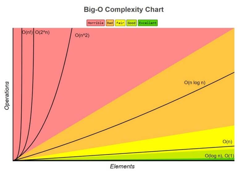
Complexity Growth Illustration from Big O Cheatsheet
Since this was only a brief introduction, there is still much to learn about algorithms. By visiting websites like Leetcode, you can hone your ability to create sound algorithms and become ready for your career as a developer. Leetcode undoubtedly benefited me and my friends, and I do not doubt that it would also benefit you. The secret to your success is consistency, so keep practicing consistently. I sincerely hope you find this as entertaining to read as I did to write it. Continue coding and lighting. PEACE.